+44 (0) 1223 755950
+1 832 327 7413
If you are using a Competitive Inhibition kit, please view our Competitive Inhibition ELISA Standard Curve Guide.
Enzyme linked immunosorbent assay (ELISA) can be used for the detection of target antigen. There are four types of ELISA: direct ELISA, indirect ELISA, sandwich ELISA and competitive inhibition ELISA. The most widely used ELISA type is the Sandwich ELISA, where the analyte is sandwiched between two antibodies, the capture antibody and the detection antibody. Results can collected by measuring the absorbance, where a high absorbance is indicative of a high concentration, and vice versa.
The standard curve is used to determine the concentration of the samples. In the example below, the standard absorbance values for abx155737, Rat IL6 ELISA Kit, are shown as a reference. As shown in Figure 1, the standard was diluted from 100 pg/ml to 1.56 pg/ml. A negative control is also run. This contains no standard (0 pg/ml). To accurately determine the true absorbance of any well, the background must be subtracted. This will give the corrected absorbance values.
| Well | Concentration of standard (pg/ml) | Absorbance | Corrected |
| A | 0 | 0.115 | 0 |
| B | 1.56 | 0.296 | 0.181 |
| C | 3.12 | 0.372 | 0.257 |
| D | 6.25 | 0.459 | 0.344 |
| E | 12.5 | 0.684 | 0.569 |
| F | 25 | 1.14 | 1.025 |
| G | 50 | 1.917 | 1.802 |
| H | 100 | 3.148 | 3.033 |
Figure 1. Data of standard concentrations, absorbance values and corrected absorbance values
Next, the O.D. value of the standard (X-axis) can be plotted against the known concentration of the standard (Y-axis), as an XY scatter plot. In the example, these values are highlighted in green in Figure 1. As shown in Figure 2, the X-axis is the Optical Density, and the Y-axis is the Standard Concentration in pg/ml.

Figure 2. Plot of 7-point XY scatter
A polynomial order 2 trendline can be added to the graph. In Excel, this can be achieved by selecting any point in the XY scatter graph, right-clicking and selecting “Add Trendline”. The trendline formatting should then be amended to polynomial order 2 (the default trendline is linear) as shown in Figure 3 below. In the formatting section, further select “Display Equation on chart” and “Display R-squared value on chart”. Excel will then display the corresponding trendline formula and R-squared value on the graph. This is shown in Figure 4 below.
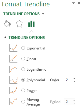
Figure 3. Addition and formatting of the trendline

Figure 4. Schematic diagram of a typical standard curve with trendline, equation and R-squared
In general, a good standard curve should have the following characteristics:
| Problem | Possible Source | Correction |
| Poor background | Contaminated negative control well | Change and use new pipette tips, containers and sealers |
| Poor R-squared | Improper standard curve preparation | Ensure accurate dilution procedure |
| Improper standard curve | Ensure accurate dilution of the standard | |
| Inaccurate Pipetting | Check and Calibrate pipettes | |
| Reused pipette tips, containers and sealers | Change and use new pipette tips, containers and sealers | |
| Low OD Values | Improper standard curve preparation | Ensure accurate operation of the dilution |
| Improper standard curve dilution | Ensure accurate dilution of the dilution | |
| Inaccurate Pipetting | Check and Calibrate pipettes | |
| Incorrect incubation times | Ensure sufficient incubation times | |
| Incorrect incubation temperature | Reagents balanced to room temperature | |
| Conjugate or substrate reagent failure | Mix conjugate and substrate; color should develop immediately | |
| No stop solution added | Follow the assay protocol in the kit manual |